SyntaxLab
Does your school support how students learn?
A spatial syntax lab. Drop in a floor plan — get a scored diagnosis in seconds.
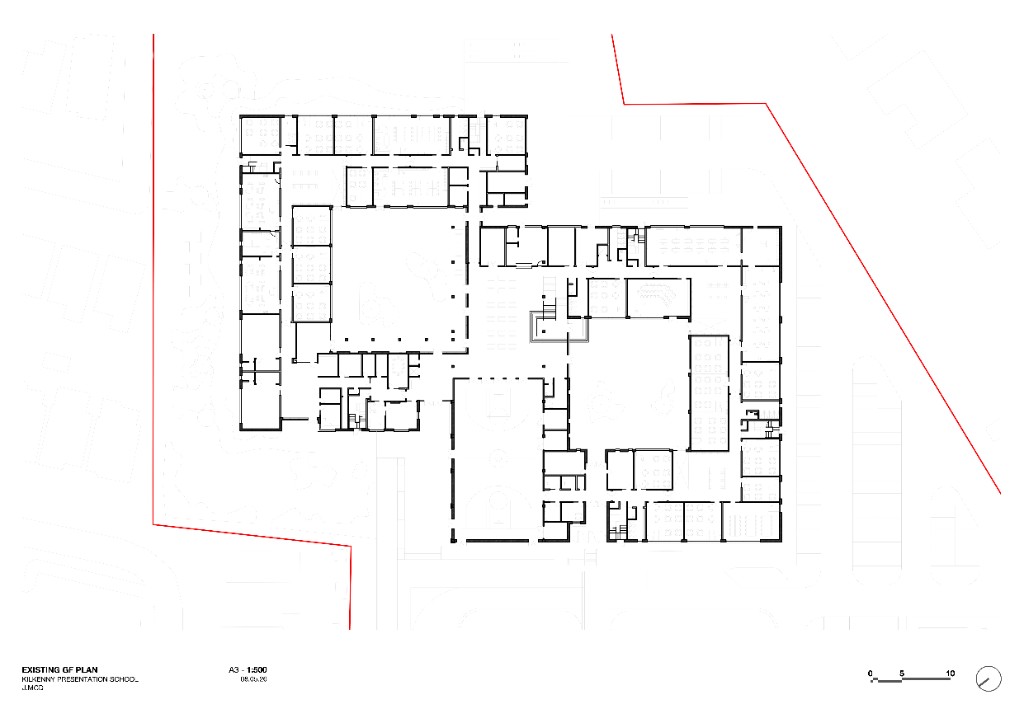
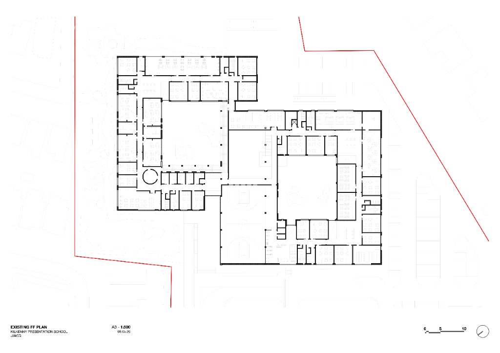
Floor Plan
Your school's rooms and how they connect to each other
→
Spatial Analysis
The tool maps social connections and wall openness room by room
→
Social Index34%
Permeability12%
Compliance18%
Benchmark 70%
Score
Each room and the whole building is scored with the same syntax rules
Reference calibration includes schools such as Kastelli (Oulu) and Hellerup (Copenhagen) —
with documented improvements in student wellbeing and learning outcomes.
with documented improvements in student wellbeing and learning outcomes.
SyntaxLab
Analysing SS Kilkenny
Reading room layout…